Ever wondered how the Variational Autoencoder (VAE) model works? Do you want to know how VAE is able to generate new examples similar to the dataset it was trained on?
After reading this post, you'll be equipped with the theoretical understanding of the inner workings of VAE, as well as being able to implement one yourself.
In a future post I'll provide you with a working code of a VAE trained on a dataset of handwritten digits images, and we’ll have some fun generating new digits!
Generative models
VAE is a generative model - it estimates the Probability Density Function (PDF) of the training data. If such a model is trained on natural looking images, it should assign a high probability value to an image of a lion. An image of random gibberish on the other hand should be assigned a low probability value.
The VAE model can also sample examples from the learned PDF, which is the coolest part, since it’ll be able to generate new examples that look similar to the original dataset!
I'll explain the VAE using the MNIST handwritten digits dataset. The input to the model is an image in $\mathbb{R}^{28×28}$. The model should estimate a high probability value if the input looks like a digit.
The challenge of modeling images
The interactions between pixels pose a great challenge. If the pixels were independent of each other, we would have needed to learn the PDF of every pixel independently, which is easy. The sampling would have been a breeze too - we would have just sampled each pixel independently.
In digit images there are clear dependencies between pixels. If you look at the left half of an image and see the start of a 4, you’d be very surprised to see the right half is the end of a 0. But why?...
Latent space
You know every image of a digit should contain, well, a single digit. An input in $\mathbb{R}^{28×28}$ doesn’t explicitly contain that information. But it must reside somewhere... That somewhere is the latent space.

You can think of the latent space as $\mathbb{R}^{k}$ where every vector contains $k$ pieces of essential information needed to draw an image. Let’s say the first dimension contains the number represented by the digit. The second dimension can be the width. The third - the angle. And so on.
We can think of the process that generated the images as a two steps process. First the person decides - consciously or not - all the attributes of the digit he’s going to draw. Next, these decisions transform into brushstrokes.
VAE tries to model this process: given an image $x$, we want to find at least one latent vector which is able to describe it; one vector that contains the instructions to generate $x$. Formulating it using the law of total probability, we get $P(x) = \int P(x|z)P(z)dz$.
Let’s pour some intuition into the equation:
- The integral means we should search over the entire latent space for candidates.
- For every candidate $z$, we ask ourselves: can $x$ be generated using the instructions of $z$? Is $P(x|z)$ big enough? If, for instance, $z$ encodes the information that the digit is 7, then an image of 8 is impossible. An image of 1, however, might be possible, since 1 and 7 look similar.
- We found a good $z$? Good! But wait a second… Is this $z$ even likely? Is $P(z)$ big enough? Let’s consider a given image of an upside down 7. A latent vector describing a similar looking 7 where the angle dimension is set to 180 degrees will be a perfect match. However, that $z$ is not likely, since usually digits are not drawn in a 180 degrees angle.
The VAE training objective is to maximize $P(x)$. We’ll model $P(x|z)$ using a multivariate Gaussian $\mathcal{N}(f(z), \sigma^2 \cdot I)$.
$f(z)$ will be modeled using a neural network. $\sigma$ is a hyperparameter that multiplies the identity matrix $I$.
You should keep in mind that $f$ is what we'll be using when generating new images using a trained model. Imposing a Gaussian distribution serves for training purposes only. If we'd use a Dirac delta function (i.e. $x = f(z)$ deterministically), we wouldn't be able to train the model using gradient descent!
The wonders of latent space
There are two big problems with the latent space approach:
- What information does each dimension hold? Some dimensions might relate to abstract pieces of information, e.g. style. Even if it was easy to interpret all dimensions, we wouldn’t want to assign labels to the dataset. This approach wouldn't scale to new datasets.
- The latent space might be entangled, i.e. the dimensions might be correlated. A digit being drawn really fast, for instance, might result in both angled and thinner brushstrokes. Specifying these dependencies is hard.
Deep learning to the rescue
It turns out every distribution can be generated by applying a sufficiently complicated function over a standard multivariate Gaussian.
Hence, we'll choose $P(z)$ to be a standard multivariate Gaussian. $f$, being modeled by a neural network, can thus be broken to two phases:
- The first layers will map the Gaussian to the true distribution over the latent space. We won't be able to interpret the dimensions, but it doesn't really matter.
- The later layers will then map from the latent space to $P(x|z)$.
So how do we train this beast?
The formula for $P(x)$ is intractable, so we’ll approximate it using Monte Carlo method:
- Sample $\{z_i\}_{i=1}^n$ from the prior $P(z)$.
- Approximate using $ P(x) \approx \frac{1}{n}\sum_{i=1}^n P(x|z_i)$.
Great! So we just sample a bunch of $z$’s and let the backpropagation party begin!
Unfortunately, since $x$ has high dimensionality, many samples are needed to get a reasonable approximation. I mean, if you sample $z$'s, what are the chances you’ll end up with an image that looks anything to do with x? This, by the way, explains why $P(x|z)$ must assign a positive probability value to any possible image, or otherwise the model won’t be able to learn: a sampled $z$ will result with an image that is almost surely different from $x$, and if the probability will be 0 the gradients won’t propagate.
So how do we solve this mess?
Let’s take a shortcut!

Most sampled $z$’s won’t contribute anything to $P(x)$ - they’ll be too off. If only we could know in advance where to sample from...
We can introduce $Q(z|x)$. $Q$ will be trained to give high probability values to $z$’s that are likely to have generated $x$. Now we can calculate the Monte Carlo estimation using much fewer samples from $Q$.
Unfortunately, a new problem arises! Instead of maximizing $P(x) = \int P(x|z)P(z)dz = \mathbb{E}_{z \sim P(z)} P(x|z)$, we’ll be maximizing $\mathbb{E}_{z \sim Q(z|x)} P(x|z)$. How do the two relate to each other?
Variational Inference
Variational Inference is a topic for a post of its own, so I won’t elaborate here. All I’ll say is that the two do relate via this equation:
$log P(X) - \mathcal{KL}[Q(z|x) || P(z|x)] = \mathbb{E}_{z \sim Q(z|x)}[log P(x|z)] - \mathcal{KL}[Q(z|x) || P(z)]$
$\mathcal{KL}$ is the Kullback–Leibler divergence, which intuitively measures how similar two distributions are.
In a moment you'll see how we can maximize the right side of the equation. By doing so, the left side will also be maximized:
- $P(x)$ will be maximized.
- how off $Q(z|x)$ is from $P(z|x)$ - the true posterior which we don't know - will be minimized.
The intuition behind the right side of the equation is that we have a tension:
- In one hand we want to maximize how well $x$ is expected to be decoded from $z \sim Q$.
- On the other hand, we want $Q(z|x)$ (the encoder) to be similar to the prior $P(z)$ (a multivariate Gaussian). One can think of this term as a regularization.
Minimizing the KL divergence is easy given the right choice of distributions. We’ll model $Q(z|x)$ as a neural network whose output is the parameters of a multivariate Gaussian:
- a mean $\mu_Q$
- a diagonal covariance matrix $\Sigma_Q$
The KL divergence then becomes analytically solvable, which is great for us (and the gradients).
The decoder part is a bit trickier. Naively, we’d tackle the fact it’s intractable by using Monte Carlo. But sampling $z$’s from $Q$ won’t allow the gradients to propagate through $Q$, because sampling is not a differentiable operation. This is problematic, since the weights of the layers that output $\Sigma_Q$ and $\mu_Q$ won’t be updated.
The reparameterization trick
We can substitute $Q$ with a deterministic parameterized transformation of a parameterless random variable:
- Sample from a standard (parameterless) Gaussian.
- Multiply the sample by the square root of $\Sigma_Q$.
- Add $\mu_Q$ to the result.
The result will have a distribution equal to $Q$. Now the sampling operation will be from the standard Gaussian. Hence, the gradients will be able to propagate through $\Sigma_Q$ and $\mu_Q$, since these are deterministic paths now.
The result? The model will be able to learn how to adjust $Q$’s parameters: it’ll concentrate around good $z$’s that are able to produce $x$.
Connecting the dots
The VAE model can be hard to grasp. We covered a lot of material here, and it can be overwhelming.
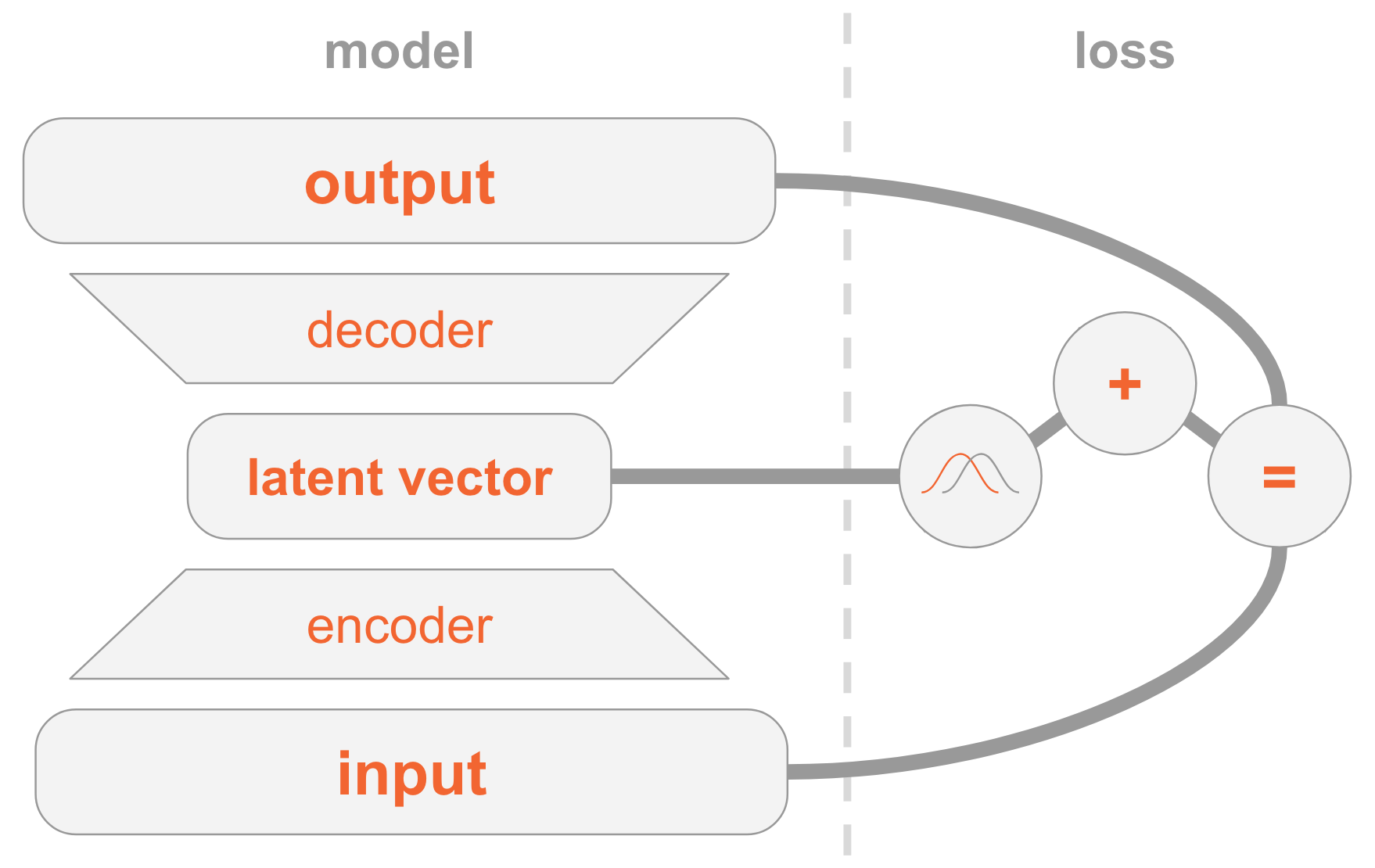
So let me summarize all the steps one needs to grasp in order to implement VAE.

On the left side we have the model definition:
- An input image is passed through an encoder network.
- The encoder outputs parameters of a distribution $Q(z|x)$.
- A latent vector $z$ is sampled from $Q(z|x)$. If the encoder learned to do its job well, most chances are $z$ will contain the information describing $x$.
- The decoder decodes $z$ into an image.
On the right side we have the loss:
- Reconstruction error: the output should be similar to the input.
- $Q(z|x)$ should be similar to the prior (multivariate standard Gaussian).
In order to generate new images, you can directly sample a latent vector from the prior distribution, and decode it into an image.
In the next post I'll provide you with a working code of a VAE. Additionally, I'll show you how you can use a neat trick to condition the latent vector such that you can decide which digit you want to generate an image for. So stay tuned :)
Notes
This post is based on my intuition and these sources:
Comments !