The Variational Autoencoder (VAE) is a paragon for neural networks that try to learn the shape of the input space. Once trained, the model can be used to generate new samples from the input space.
If we have labels for our input data, it’s also possible to condition the generation process on the label. In the MNIST case, it means we can specify which digit we want to generate an image for.
Let’s take it one step further... Could we condition the generation process on the digit without using labels at all? Could we achieve the same results using an unsupervised approach?
If we wanted to rely on labels, we could do something embarrassingly simple. We could train 10 independent VAE models, each using images of a single digit.
That would obviously work, but you're using the labels. That's cheating!
OK, let’s not use them at all. Let’s train our 10 models, and just, well, have a look with our eyes on each image before passing it to the appropriate model.
Hey, you’re cheating again! While you don’t use the labels per se, you do look at the images in order to route them to the appropriate model.
Fine... If instead of doing the routing ourselves we let another model learn the routing, that wouldn’t be cheating at all, would it?
Right! :)
We can use an architecture of 11 modules as follows:
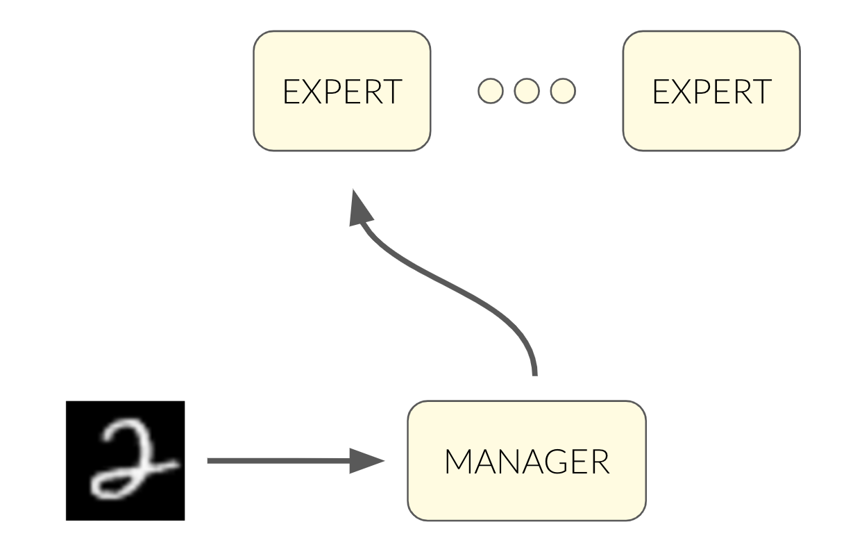
But how will the manager decide which expert to pass the image to? We could train it to predict the digit of the image, but again - we don’t want to use the labels!
Phew... I thought you're gonna cheat...
So how can we train the manager without using the labels? It reminds me of a different type of model - Mixture of Experts (MoE). Let me take a small detour to explain how MoE works. We'll need it, since it's going to be a key component of our solution.
Mixture of Experts explained to non-experts
MoE is a supervised learning framework. You can find a great explanation by Geoffrey Hinton on Coursera and on YouTube. MoE relies on the possibility that the input might be segmented according to the $x \rightarrow y$ mapping. Have a look at this simple function:
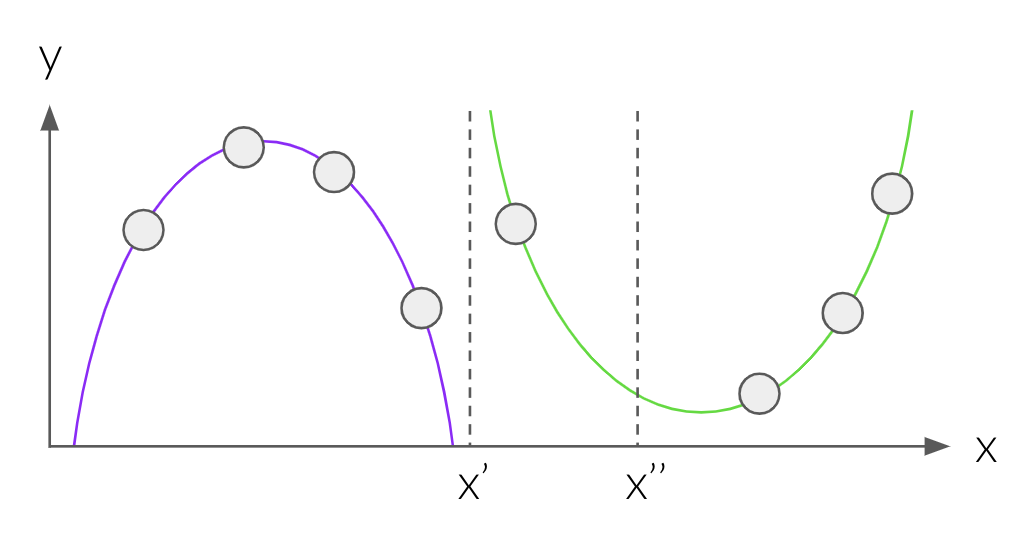
The ground truth is defined to be the purple parabola for $x < x$', and the green parabola for $x >= x$'. If we were to specify by hand where the split point $x$' is, we could learn the mapping in each input segment independently using two separate models.
In complex datasets we might not know the split points. One (bad) solution is to segment the input space by clustering the $x$’s using K-means. In the two parabolas example, we’ll end up with $x$'' as the split point between two clusters. Thus, when we’ll train the model on the $x < x$'' segment, it’ll be inaccurate.
So how can we train a model that learns the split points while at the same time learns the mapping that defines the split points?
MoE does so using an architecture of multiple subnetworks - one manager and multiple experts:
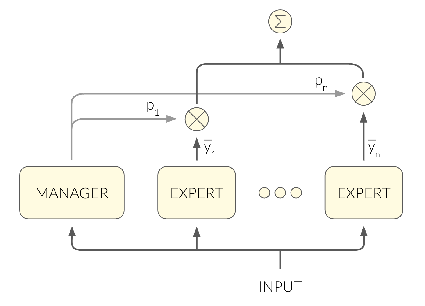
The manager maps the input into a soft decision over the experts, which is used in two contexts:
- The output of the network is a weighted average of the experts’ outputs, where the weights are the manager’s output.
The loss function is $\sum_i p_i(y - \bar{y_i})^2$. $y$ is the label, $\bar{y_i}$ is the output of the i'th expert, $p_i$ is the i'th entry of the manager's output. When you differentiate the loss, you get these results (I encourage you to watch the video for more details):
- The manager decides for each expert how much it contributes to the loss. In other words, the manager chooses which experts should tune their weights according to their error.
The manager tunes the probabilities it outputs in such a way that the experts that got it right will get higher probabilities than those that didn’t.
This loss function encourages the experts to specialize in different kinds of inputs.
The last piece of the puzzle... is $x$
Let’s get back to our challenge! MoE is a framework for supervised learning. Surely we can change $y$ to be $x$ for the unsupervised case, right? MoE's power stems from the fact that each expert specializes in a different segment of the input space with a unique mapping $x \rightarrow y$. If we use the mapping $x \rightarrow x$, each expert will specialize in a different segment of the input space with unique patterns in the input itself.
We'll use VAEs as the experts. Part of the VAE’s loss is the reconstruction loss, where the VAE tries to reconstruct the original input image $x$:
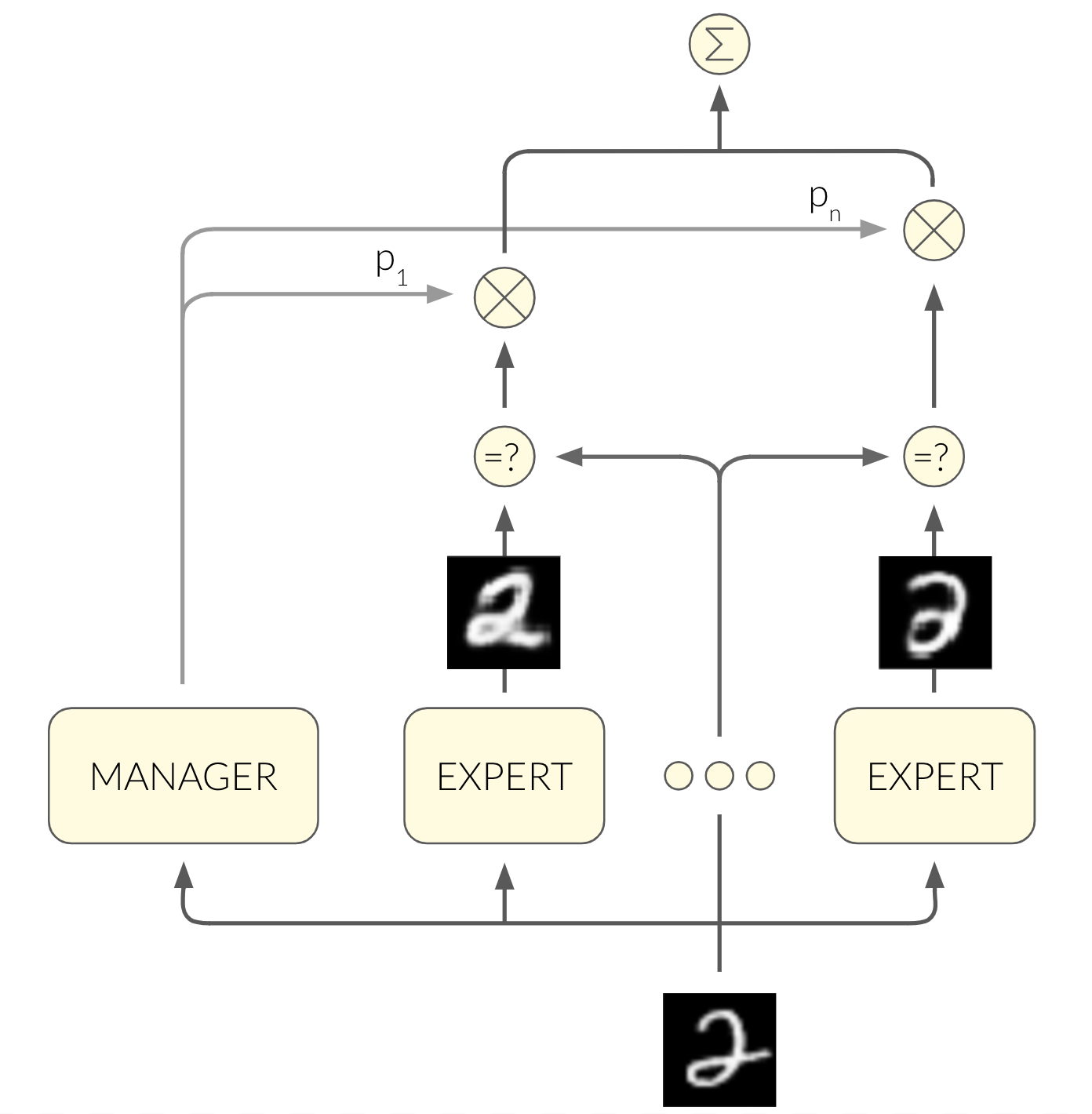
A cool byproduct of this architecture is that the manager can classify the digit found in an image using its output vector!
One thing we need to be careful about when training this model is that the manager could easily degenerate into outputting a constant vector - regardless of the input in hand. This results in one VAE specialized in all digits, and nine VAEs specialized in nothing. One way to mitigate it, which is described in the MoE paper, is to add a balancing term to the loss. It encourages the outputs of the manager over a batch of inputs to be balanced: $\sum_\text{examples in batch} \vec{p} \approx Uniform$.
Enough talking - It's training time!
import numpy as np
import tensorflow as tf
from tensorflow.examples.tutorials.mnist import input_data
import matplotlib.pyplot as plt

np.random.seed(42)
tf.set_random_seed(42)

%matplotlib inline
mnist = input_data.read_data_sets('MNIST_data')
INPUT_SIZE = 28 * 28
NUM_DIGITS = 10
params = {
    'manager_layers': [128],        # the manager will be implemented using a simple feed forward network
    'encoder_layers': [128],        # ... and so will be the encoder
    'decoder_layers': [128],        # ... and the decoder as well (CNN will be better, but let's keep it concise)
    'activation': tf.nn.sigmoid,    # the activation function used by all subnetworks
    'decoder_std': 0.5,             # the standard deviation of P(x|z) discussed in the first post of the series
    'z_dim': 10,                    # the dimension of the latent space
    'balancing_weight': 0.1,        # how much the balancing term will contribute to the loss
    'epochs': 100,
    'batch_size': 100,
    'learning_rate': 0.001
}
class VAE(object):
    _ID = 0

    def __init__(self, params, images):
        self._id = VAE._ID
        VAE._ID += 1
        self._params = params
        encoder_mu, encoder_var = self.encode(images)

        eps = tf.random_normal(shape=[tf.shape(images)[0],
                                      self._params['z_dim']],
                               mean=0.0,
                               stddev=1.0)
        z = encoder_mu + tf.sqrt(encoder_var) * eps

        self.decoded_images = self.decode(z)
        self.loss = self._calculate_loss(images,
                                         self.decoded_images,
                                         encoder_mu,
                                         encoder_var)


    def encode(self, images):
        with tf.variable_scope('encode_{}'.format(self._id), reuse=tf.AUTO_REUSE):
            x = images
            for layer in self._params['encoder_layers']:
                x = tf.layers.dense(x,
                                    layer,
                                    activation=self._params['activation'])
            mu = tf.layers.dense(x, self._params['z_dim'])
            var = 1e-5 + tf.exp(tf.layers.dense(x, self._params['z_dim']))
        return mu, var


    def decode(self, z):
        with tf.variable_scope('decode_{}'.format(self._id), reuse=tf.AUTO_REUSE):
            for layer in self._params['decoder_layers']:
                z = tf.layers.dense(z,
                                    layer,
                                    activation=self._params['activation'])
            mu = tf.layers.dense(z, INPUT_SIZE)
        return tf.nn.sigmoid(mu)


    def _calculate_loss(self, images, decoded_images, encoder_mu, encoder_var):
        loss_reconstruction = -tf.reduce_sum(
            tf.contrib.distributions.Normal(
                decoded_images,
                self._params['decoder_std']
            ).log_prob(images),
            axis=1
        )

        loss_prior = -0.5 * tf.reduce_sum(
            1 + tf.log(encoder_var) - encoder_mu ** 2 - encoder_var,
            axis=1
        )

        return loss_reconstruction + loss_prior
class Manager(object):
    def __init__(self, params, experts, images):
        self._params = params
        self._experts = experts
        probs = self.calc_probs(images)
        self.expected_expert_loss, self.balancing_loss, self.loss = self._calculate_loss(probs)


    def calc_probs(self, images):
        with tf.variable_scope('prob', reuse=tf.AUTO_REUSE):
            x = images
            for layer in self._params['manager_layers']:
                x = tf.layers.dense(x,
                                    layer,
                                    activation=self._params['activation'])
            logits = tf.layers.dense(x, len(self._experts))
            probs = tf.nn.softmax(logits)
        return probs


    def _calculate_loss(self, probs):
        losses = tf.concat([tf.reshape(expert.loss, [-1, 1])
                            for expert in self._experts], axis=1)
        expected_expert_loss = tf.reduce_mean(tf.reduce_sum(losses * probs, axis=1), axis=0)
        experts_importance = tf.reduce_sum(probs, axis=0)
        _, experts_importance_var = tf.nn.moments(experts_importance, axes=[0])
        balancing_loss = experts_importance_var
        loss = expected_expert_loss + self._params['balancing_weight'] * balancing_loss
        return expected_expert_loss, balancing_loss, loss
images = tf.placeholder(tf.float32, [None, INPUT_SIZE])
experts = [VAE(params, images) for _ in range(NUM_DIGITS)]
manager = Manager(params, experts, images)

train_op = tf.train.AdamOptimizer(params['learning_rate']).minimize(manager.loss)
samples = []
expected_expert_losses = []
balancing_losses = []
losses = []
with tf.Session() as sess:
    sess.run(tf.global_variables_initializer())
    for epoch in range(params['epochs']):
        # train over the batches
        for _ in range(mnist.train.num_examples / params['batch_size']):
            batch_images, batch_digits = mnist.train.next_batch(params['batch_size'])
            sess.run(train_op, feed_dict={images: batch_images})

        # keep track of the loss
        expected_expert_loss, balancing_loss, loss = sess.run(
            [manager.expected_expert_loss, manager.balancing_loss, manager.loss],
            {images: mnist.train.images}
        )
        expected_expert_losses.append(expected_expert_loss)
        balancing_losses.append(balancing_loss)
        losses.append(loss)

        # generate random samples so we can have a look later on
        sample_z = np.random.randn(1, params['z_dim'])
        gen_samples = sess.run([expert.decode(tf.constant(sample_z, dtype='float32'))
                                for expert in experts])
        samples.append(gen_samples)
plt.subplot(131)
plt.plot(expected_expert_losses)
plt.title('expected expert loss', y=1.07)

plt.subplot(132)
plt.plot(balancing_losses)
plt.title('balancing loss', y=1.07)

plt.subplot(133)
plt.plot(losses)
plt.title('total loss', y=1.07)

plt.tight_layout()

def plot_samples(samples, num_epochs):
    IMAGE_WIDTH = 0.7
    epochs = np.linspace(0, len(samples) - 1, num_epochs).astype(int)
    plt.figure(figsize=(IMAGE_WIDTH * NUM_DIGITS,
                        len(epochs) * IMAGE_WIDTH))
    for epoch_index, epoch in enumerate(epochs):
        for digit, image in enumerate(samples[epoch]):
            plt.subplot(len(epochs),
                        NUM_DIGITS,
                        epoch_index * NUM_DIGITS + digit + 1)
            plt.imshow(image.reshape((28, 28)),
                       cmap='Greys_r')
            plt.gca().xaxis.set_visible(False)
            if digit == 0:
                plt.gca().yaxis.set_ticks([])
                plt.ylabel('epoch {}'.format(epoch + 1),
                           verticalalignment='center',
                           horizontalalignment='right',
                           rotation=0,
                           fontsize=14)
            else:
                plt.gca().yaxis.set_visible(False)


plot_samples(samples=samples, num_epochs=20)

In the last figure we see what each expert has learned. After each epoch we used the experts to generate images from the distributions they specialized in. The i’th column contains the images generated by the i’th expert.
We can see that some of the experts easily managed to specialize in a single digit, e.g. - 1. Some got a bit confused by similar digits, such as the expert that specialized in both 3 and 5.
 An expert specializing in 2
What else?
Using a simple model without a lot of tuning and tweaking, we got reasonable results. Optimally, we would want each expert to specialize in exactly one digit, thus achieving a perfect unsupervised classification via the output of the manager.
Another interesting experiment would be to turn each expert into a MoE of its own! It will allow us to learn hierarchical parameters by which VAEs should specialize. For instance, some of the digits have multiple ways to be drawn: 7 can be drawn with or without a strikethrough line. This source of variation could be modeled by the MoE in the second level of the hierarchy. But I’ll leave something for a future post...
Comments !